A History of Humanity's Quest for the Best Answer

The Unchanging Problem

We tend to tell the story of scientific progress, and of AI along with it, as a sequence of brand-new problems. This essay takes the opposite view: underneath it all sits one problem that never changes, only the mathematical tools brought to bear on it get more sophisticated, and more daring. That one problem is optimization.

At bottom, the task hasn't shifted at all. Whether it's a 19th-century astronomer mapping the sky or a modern neural network learning to recognize a photo, the aim is the same: find the parameters that push a loss function, a plain measure of how wrong the model is, as low as possible. To trace that story, we'll lean on one recurring image: the "error landscape."

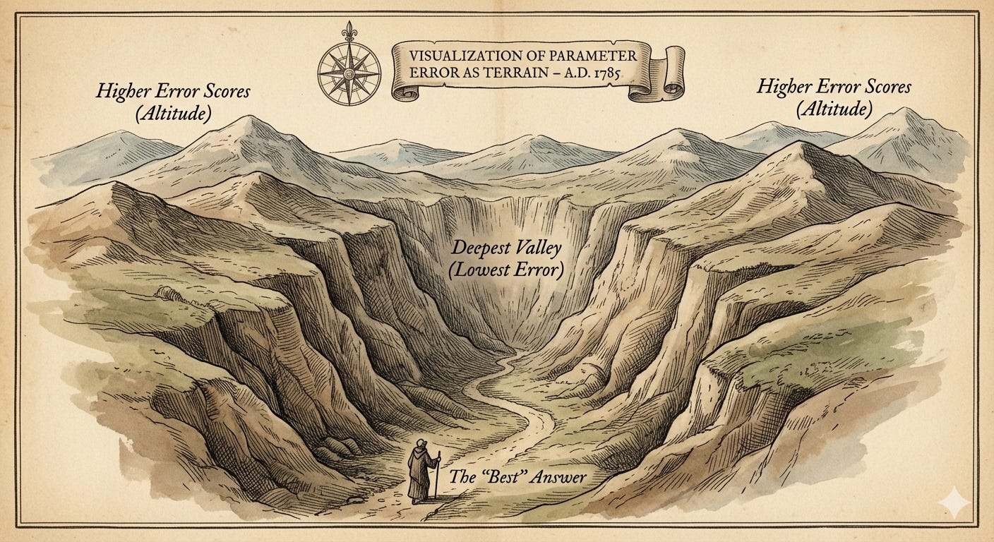
Picture every possible setting of the parameters as a point with its own altitude, its error score. The best solution sits at the lowest point, the floor of the deepest valley. What separates one era from the next isn't the wish to find that valley, everyone wants that, it's how complicated a terrain they were willing to attempt. The arc we'll follow runs from a landscape that's a single, tidy bowl to one that looks like a sprawling, chaotic mountain range.

That progression traces a deeper shift in what "getting smarter" even means. It isn't simply more raw computational muscle, it's a fundamentally different relationship with uncertainty and with the idea of a perfect answer.

• Era I, the 1800s, insisted on total, deterministic certainty: the answer had to be one exact formula, and the problem wasn't "solved" until you could prove that formula was the only possible solution.
• Era II, the 1950s, made room for iteration, a step-by-step search, but only on one condition: a mathematical guarantee that the search would land on the single best answer. That guarantee, convexity, was what let people trust these unfamiliar new electronic computers.
• Era III, the 2010s, took a braver step: it let go of any guarantee of optimality and settled for "good enough" in landscapes so tangled (non-convex) that a truly optimal answer wasn't even knowable.
• Era IV, still ahead of us, is learning to operate with almost no signal to follow at all, a landscape with no gradient, relying on pure black-box trial and error to crack problems that were previously out of reach.

So "getting smarter," in practice, has meant a slow and fairly bold retreat from the need for perfect certainty. It's precisely that willingness to let go that lets us take on problems that are messier, more complex, and closer to how the real world actually behaves.

As a scaffold for the rest of this piece, here's a quick summary of the four eras of optimization.

Part I An Age of Certainty: Exact Answers for a Clockwork Universe (the 1800s)

The Story: A Planet Goes Missing

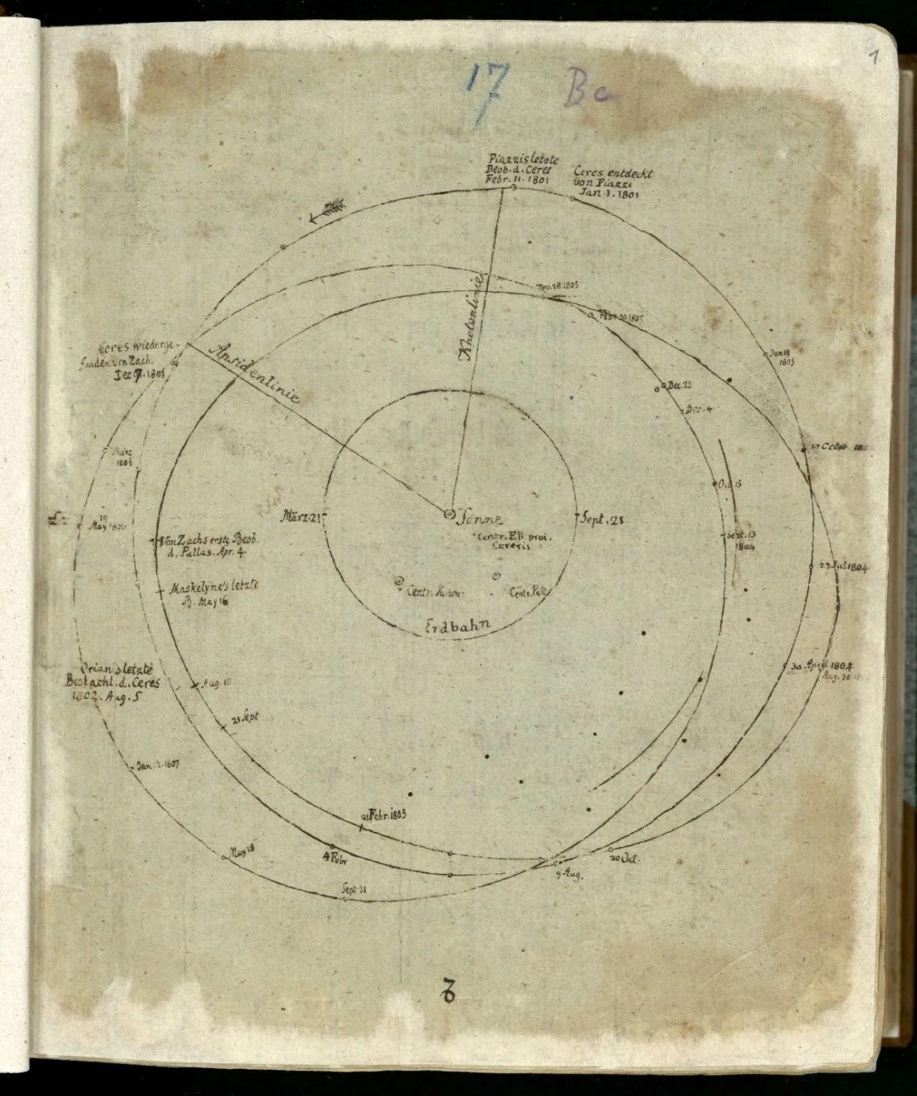
Optimization's life as a practical, working tool doesn't start with a computer, it starts with a crisis in the sky. On New Year's Day 1801, Giuseppe Piazzi, observing from Palermo, spotted a celestial object nobody had seen before. He tracked it carefully for forty days, but lost it again before he could pin down its orbit, swallowed by the glare of the sun.

This wasn't just any missing object, astronomers were gripped by it. Its position matched the Titius-Bode law, a rule predicting how planets should be spaced, right in the gap between Mars and Jupiter where a planet was "supposed" to be. Recovering it became one of the era's defining scientific challenges. The trouble was that it looked impossible: how do you reconstruct a full elliptical orbit from a handful of sparse, noisy observations?

The answer came from Carl Friedrich Gauss, then just 24. He'd quietly been refining a powerful technique in his private notebooks since he was 18, in 1795, without ever publishing it. Turning it loose on Piazzi's thin data, he produced a remarkably precise prediction of where the object, which he'd named Ceres, would reappear.

On December 7, 1801, Franz Xaver von Zach pointed his telescope where Gauss's math told him to, and found Ceres again. It was a genuine moment of scientific heroism, mathematics winning out over uncertainty, and it made Gauss famous well beyond Germany. The tool behind it was the method of least squares.

The Human Side: A "Trivial" Discovery and a Famous Feud

Gauss's dramatic success brought, almost inevitably, a priority dispute with another mathematical giant. He'd used the method back in 1801, but the Frenchman Adrien-Marie Legendre had arrived at it independently, and published it first. Legendre's 1805 book, Nouvelles méthodes pour la détermination des orbites des comètes, was the first public account of the technique.

What followed became one of science's best-known feuds. Legendre, first into print, considered the matter settled in his favor. Gauss, in his 1809 publication, pointed out that he'd actually been using the method since 1795, a claim that was true, and that Legendre found maddening.

The Math: A One-Step Answer

Every calculation in this era had to be worked by hand, and that constraint alone forced a philosophy built around certainty: trial-and-error search simply wasn't feasible. What Gauss and Legendre offered instead was a closed-form solution, one direct formula, no iteration, that handed you the exact final answer in a single pass.

The task was to find the parameters β, for a line or an orbit, that minimized total error. That error, L, is defined as the sum of the squared vertical gaps between what was observed and what the model predicted.

The Loss Function. Written in matrix form, this is the least-squares loss: y is the vector of observations, X the matrix of input data, and β the vector of parameters we're solving for.

The error itself, the residual, is:

Minimizing the sum of squared residuals, in matrix notation, gives:

Taking the derivative of L with respect to β (skipping the intermediate calculus) gives the gradient:

That result is the Normal Equation, and it's a remarkable thing: a direct formula for the best possible answer. No guesswork, no iterating. Feed in your observed data, X and y, run the matrix operations, and the one optimal solution falls out.

Geometrically, there's something almost elegant about it.

This term is a projection matrix, and what the formula is really doing is finding the "shadow" that your real-world data vector casts onto the idealized space defined by X. The parameters are just the recipe for that shadow. It was exactly the kind of answer suited to an age that still believed in a clockwork, fully-determined universe.

Part II An Age of Confidence: The Guaranteed Search (the 1950s)

The Story: A Problem of Scale

The arrival of the electronic computer, SEAC, built by the National Bureau of Standards in 1950, changed what optimization could even attempt. Iterative, trial-and-error calculation suddenly became practical. What it needed was a problem worthy of it, and that problem was scale. During WWII, the US Army Air Force had leaned on rooms of clerks with desk calculators to try to mechanize planning; after the war, that effort became Project SCOOP (Scientific Computation of Optimal Programs), a dedicated task force inside the Air Force.

This was no longer about locating a single planet. It was allocating thousands of resources at once, tuning factory output, routing enormous supply chains. These became known as linear programming problems, and with thousands of variables apiece, they were well beyond anything Gauss's one-step Normal Equation could touch.

The Hero, and Some "Unsolved Homework"

This era's central figure was George Dantzig, and his origin story has become something of a legend. As a Berkeley graduate student, he showed up late one day to the statistics class taught by the well-known Jerzy Neyman.

Finding two problems on the board, he took them for the homework assignment and copied them down. A few days later he turned them in late, apologizing, and mentioning they'd felt harder than usual. What he'd actually done was solve two open, unsolved problems in statistics. Neyman was impressed enough to accept the work as Dantzig's doctoral thesis.

The Tool, and the "Diet Problem"

Years on, as chief mathematician for Project SCOOP, Dantzig produced his defining achievement: the Simplex Method, built to solve exactly these large linear programming problems. First devised in 1947, it became the workhorse algorithm of the whole 1950s paradigm.

To try the method out, Dantzig famously turned it on himself: the "Diet Problem," finding the cheapest combination of foods that would satisfy all his daily nutrition needs. What came out the other end turned into a perfect, and genuinely funny, parable for the future of AI.

His wife Anne remembered him phoning home with the first "optimal" answer. He admitted it was a bit strange: it called for drinking a couple of gallons of vinegar a day.

It turned out a data-entry mistake had listed vinegar as extremely nutritious. With that fixed and the program rerun, Dantzig called again with a new answer, this one, he promised, was reasonable: 200 bouillon cubes a day. His wife answered with one of the more memorable puns in the history of science: "What are you trying to do, corner the bouillon market?"

There's more to this story than comedy. It may be the earliest real example of an "alignment failure." The algorithm itself was flawless, it did precisely what it was asked. The problem sat in Dantzig's objective function, the constraints, which never capped salt intake. Simplex simply exposed that gap without mercy. It's a fitting origin story for a core idea in AI safety: an optimizer chases the goal you actually specified, not the one you had in mind, and a flawed objective, optimized well, can do more damage than no optimization at all.

The Concept: Convexity as a Safety Net

The new computers could iterate, but that raised a question: how could Dantzig trust Simplex to actually work? The search space was enormous. What if it settled into a false valley, a solution that looked good, a local minimum, without being the true best answer, the global minimum?

The answer the 1950s leaned on was a mathematical safety net of a different kind of certainty: convexity.

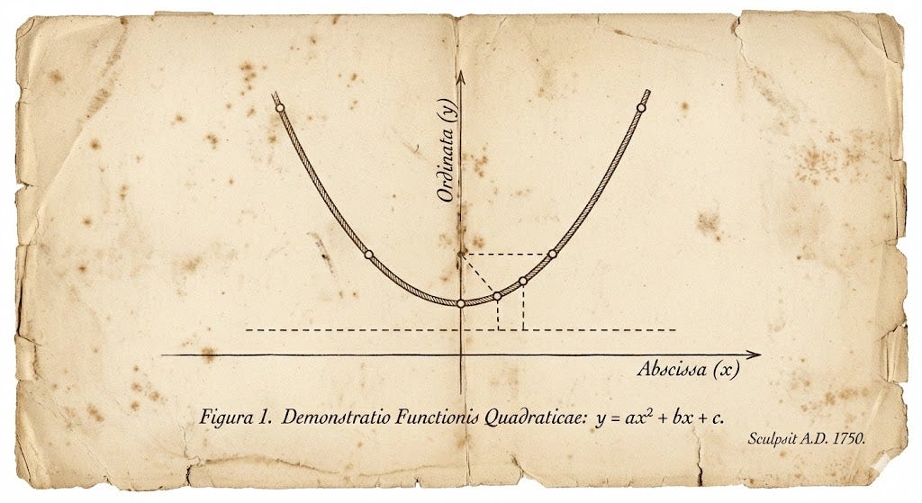
A function counts as convex when its error landscape forms one clean, simple bowl, no dips, no false bottoms, just a single smooth basin.

The formal test for that bowl shape is simple and rather elegant: pick any two points on the function's graph, draw a straight line between them, and that line will never fall below the curve itself.

The Diet Problem, cheapest food combination meeting minimum nutrition, was a fundamentally different kind of challenge from Gauss's. It's a constrained optimization problem, shaped by linear inequalities (Dantzig, 1990). Rather than reconciling conflicting data, the goal is to find the best outcome achievable inside a fixed set of boundaries.

The Diet Problem is a textbook Linear Programming (LP) problem, which in its standard form looks like this:

subject to the nutritional constraints:

Here x_i is how much of food i you eat, c_i its price per unit, b_j the minimum required amount of nutrient j, and a_ij how much of nutrient j sits in one unit of food i.

Simplex was Dantzig's systematic way of solving this. Every LP problem defines a "feasible region," a convex, many-sided shape (a polyhedron) formed by the intersection of all its constraints. Dantzig's key insight, the Fundamental Theorem of Linear Programming, was that if an optimal solution exists at all, it sits at one of that shape's corners. Simplex simply walks along the polyhedron's edges, corner to better corner, until no improvement is left. It was the first practical way to handle large, heavily constrained planning problems, and it effectively founded the field of Operations Research.

Its descendants are everywhere: logistics firms use it to find the cheapest routing for thousands of shipments, refineries use it to blend crude oil into gasoline and jet fuel, and financial firms use it to balance portfolios against risk. Problems with hundreds of variables and constraints were essentially unsolvable before Simplex; Dantzig's method made them tractable, and opened up the modern era of operations research.

Part III An Age of Pragmatism: Taming the Non-Convex (the 2010s)

The Story: The ImageNet Moment

Skip ahead sixty years. The problem is no longer plotting orbits or scheduling factories, it's teaching a machine to see. Specifically: the ImageNet Large Scale Visual Recognition Challenge, sorting 1.2 million high-resolution photos correctly into a thousand categories, everything from "Maltese dog" to "container ship" to "lemon."

Here the error landscape is nothing like a tidy convex bowl. It's a highly irregular, non-convex mountain range, with billions of parameters and more hills, saddle points, and valleys than anyone could count.

2012 broke the problem wide open. AlexNet, a deep network from Alex Krizhevsky, Ilya Sutskever, and Geoffrey Hinton, won the challenge, and not by a small margin: 15.3% error against 26.2% for the best non-deep-learning entry. That's not a win, it's a revolution, arguably the Big Bang of the modern AI era, and nothing looked the same afterward.

The Tool, and Its Sleeper History

What new optimization engine drove this breakthrough? Ironically, none. The engine was a sixty-year-old method with a reputation for being sloppy and imprecise: Stochastic Gradient Descent (SGD).

The Humble Origin: 1951. The core idea, approximating a true gradient stochastically, traces back to the 1951 Robbins-Monro algorithm. It was a known statistical tool, though never a dominant one, used for simple models like ADALINE linear regression in the 1960s.

The Academic Champion: 1991. For decades SGD lived in the shadow of fancier, theoretically faster optimization methods. Its most persistent advocate was Léon Bottou, who, starting with his 1991 paper "Stochastic Gradient Learning in Neural Networks" and continuing through papers across the 1990s and 2000s, kept making the case that whatever its theoretical speed disadvantage, SGD was dramatically more efficient and more robust for training networks on large datasets.

So why did an idea from 1951, championed in 1991, suddenly take over in 2012? Because the problem it was built for had finally shown up. SGD's real advantage is that its cost has nothing to do with total dataset size: rather than computing the true gradient across all 1.2 million ImageNet photos, an impossible amount of computation, it estimates the gradient from a small random minibatch, say, 128 images.

On the small academic datasets of the 20th century that trait barely mattered. In the Big Data era ImageNet ushered in, that same "flaw" became its greatest strength, the only realistic way to work through a dataset that size. AlexNet's win was really the coronation of a sleeper algorithm that had spent sixty years waiting for datasets, and GPUs well suited to minibatch math, big enough to actually need it.

The Concept: Why the Noise Is a Feature, Not a Bug

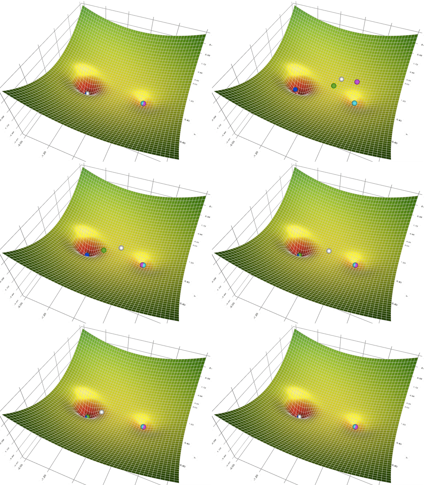
This called for a new philosophy, a pragmatic shift. In a non-convex mountain range, finding the single lowest point, the global minimum, is computationally out of reach, and it turns out you don't even want it. The 2010s approach gave up that search and settled instead for any valley that was good enough.

This is exactly where SGD's flaw turns into its magic.

• The Jiggle. Because SGD estimates the slope from a small random minibatch, its read on the "true" gradient is noisy. Rather than gliding smoothly downhill, the optimizer jiggles and oscillates as it goes.
• The Benefit: Escaping Bad Valleys. A non-convex landscape is full of bad valleys, shallow, sharp local minima that would trap a smoother optimizer. SGD's jiggle turns out to be exactly what lets it escape those shallow traps, bouncing back out and continuing on toward something deeper.
• The Flat Minima Hypothesis. Research suggests the noise does more than help with escape. It acts like a smoothing operator, blurring the error landscape so that sharp, narrow valleys effectively vanish while broad, flat ones stay visible. That pushes SGD toward settling in those wide, flat minima, and it matters, because flat minima have been shown to generalize better to data the model hasn't seen.

In short, the very sloppiness and imprecision that made SGD look second-rate in a convex world are exactly what make it so effective in the chaotic, non-convex world of deep learning.

Part IV The Next Frontier: Optimizing in the Dark (the 2030s)

The Story: A Robot's Dilemma

SGD runs the modern world, but it has one fatal weakness: it needs a smooth, differentiable error landscape to work at all. It has to be able to compute a meaningful gradient, a slope, just to know which way is downhill.

But plenty of real problems don't offer a slope at all, just an all-or-nothing result. A robot arm grasps the object or it doesn't. A self-driving car avoids the obstacle or it crashes. In control problems like these, the feedback is frequently just success or failure, and to that, SGD's gradient-based map is simply blind.

The Hurdle: The Zero-Slope Problem

The loss function we actually care about, in the real world, is the 0/1 loss: a loss of 1 when you're wrong, 0 when you're right. It isn't some abstract stand-in, it's literally accuracy, the one number that ultimately matters.

The Visual: A Step Function. So what does the 0/1 loss's landscape actually look like? Not a bowl, not a mountain range, a flat plateau at loss 1, a sheer 90-degree drop, and another flat plateau at loss 0. Just a plain step function.

The Problem: A Gradient of Zero. And the slope of a flat, horizontal line is, of course, zero.

That's the zero-slope problem, and it matters because an optimizer like SGD navigates purely by following the gradient.

• If the model is completely wrong, loss sits at 1, on the upper plateau, gradient zero.
• If it's completely right, loss sits at 0, on the lower plateau, gradient also zero.

Either way, the optimizer computes a gradient of zero and stops, convinced it has already found a minimum. It gets no signal at all telling it how to improve, or even which plateau it's actually standing on.

This is really the dirty secret, or the necessary lie, at the center of modern deep learning. Since we can't directly optimize the 0/1 loss we actually want, we optimize surrogate functions instead. Smooth, differentiable losses like cross-entropy or hinge loss aren't the real target, they're smooth stand-ins for that step function. The whole of Era III has rested on hoping that minimizing the surrogate also minimizes the real 0/1 loss. The zero-slope problem is exactly the wall you hit once that approximation stops holding up, which happens often in robotics.

A New Paradigm: Zero-Order (ZO) Optimization

If the gradient, the first-order information, is missing, useless, or actively misleading, the obvious question is: what if we just stopped relying on it? That's the philosophy behind the next frontier, zero-order (ZO) optimization.

First-Order vs. Zero-Order. This is a genuinely different philosophy about what information you need:

• First-order (SGD) needs the gradient. It's a map-based search, asking: which direction is downhill from here?
• Zero-order (ZO) is gradient-free. All it needs is the final loss value, a black-box search asking: is this new point better or worse than the last one?

The Method: "Smarter" Trial and Error. ZO methods turn optimization into a guided form of trial and error. Instead of tracing a precise path, they lean on techniques like random search or gradient approximation.

Evolutionary strategies (ES) are a good example, a family of algorithms that had their first wave of popularity in the 1970s and are now seeing a serious revival. The process itself is simple, and needs no gradient at all:

1. Generate a population: start from one parent solution, then create a population, say 100 children, by adding random noise to the parent's parameters.
2. Evaluate fitness: run all 100 children and record each one's final loss, its fitness.
3. Select and recombine: discard the 50 weakest, and average the parameters of the 50 strongest into a new parent for the next round.
4. Repeat: generation after generation, this black-box process nudges the search toward better-performing regions of the landscape, without ever touching a gradient. It's a smarter way of finding your way in the dark.

Part V — Conclusion: The Unchanging Manifold

These four eras aren't really separate histories. They're four chapters of one continuous story: the attempt to map a single "optimization manifold." The story of AI, in that sense, is the story of explorers building new tools to chart that same unchanging landscape.

The tools kept changing, and we kept getting smarter, but the intelligence was never really in the tools. It was in the nerve to use them: the willingness to give up the comfort of Gauss's certainty, the courage to leave behind the safety of Dantzig's guarantee, and now, perhaps, the willingness to abandon even the pragmatism of "good enough" in favor of the blind, unsettling uncertainty of trial and error, in service of the problems that actually matter.

1. Least squares — math.mit.edu
2. Least squares — en.wikipedia.org
3. Titius–Bode law — sites.math.rutgers.edu
4. Ceres — jpl.nasa.gov
5. Gauss — repository.lsu.edu
6. Legendre, 1805 — google.co.uk/books
7. Project SCOOP — pubsonline.informs.org
8. Dantzig / Neyman — pubsonline.informs.org
9. The Diet Problem — conversableeconomist.com
10. ImageNet / AlexNet — proceedings.neurips.cc
11. Stochastic gradient descent — fa.bianp.net
12. Bottou, 1991 — leon.bottou.org
13. SGD oscillation — lunartech.ai
14. Flat minima — arxiv.org
15. Evolution strategies — lilianweng.github.io
16. Zeroth-order optimization — emergentmind.com